Stop guessing. Start simulating.
AirInduct Sim takes you from coil geometry to coupling factor to CAD export in a single, instrumented session.
What can AirInduct Sim calculate?
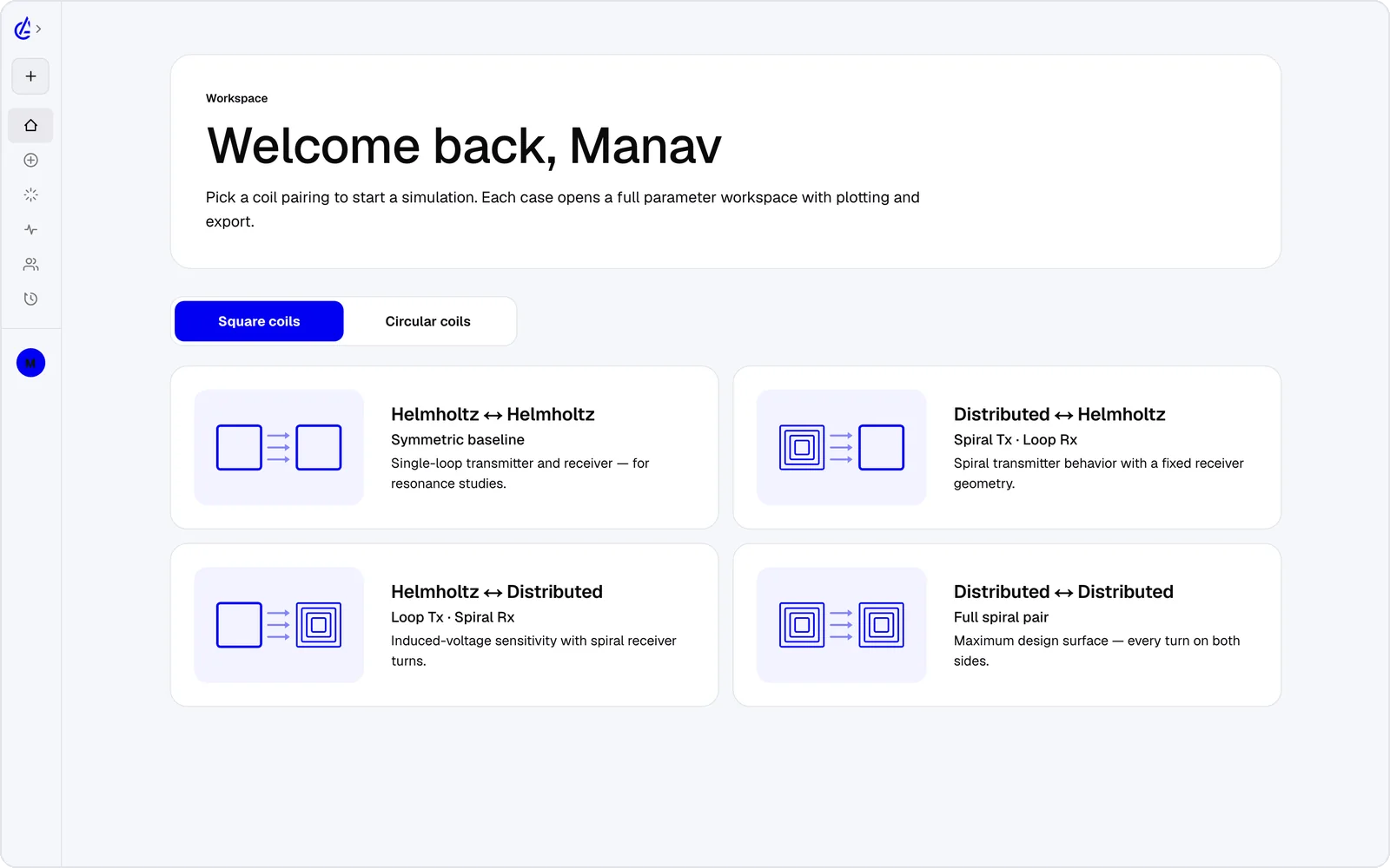
AirInduct Sim calculates the mutual inductance M, the transmitter and receiver self-inductances L_tx and L_rx, the coupling coefficient k, the induced voltage and the peak magnetic field H for a coaxial coil pair. Every value comes from closed-form Biot–Savart and Neumann integrals, so there is no mesh to build or converge. The calculators cover eight topologies: circular and square Helmholtz pairs, circular and square DTC (descending-turn planar spiral) pairs, and the four Helmholtz–DTC cross pairs. Around the solver sit the tools that turn a result into a design: 3D surface, heatmap and contour plots, parameter sweeps, an optimizer that searches for a target, and export to PDF, KiCad, DXF and SPICE. The AI Copilot adds link analysis — Q, kQ efficiency and compensation capacitors — and checks field exposure against ICNIRP and IEEE reference levels. The free plan includes the Helmholtz topology; AirInduct Pro unlocks the other seven.
Real physics. Real speed.
Vectorised Biot–Savart, Neumann mutual-inductance and elliptic-integral kernels — no FEM, no meshing, no convergence babysitting. A 100 × 100 field map returns in roughly two seconds; a 50³ volume in fifteen.
- Kernel: Biot–Savart · Neumann · K/E
- 2D: ≤ 500 × 500
- 3D: ≤ 100³
Square and circular, Helm and DTC.
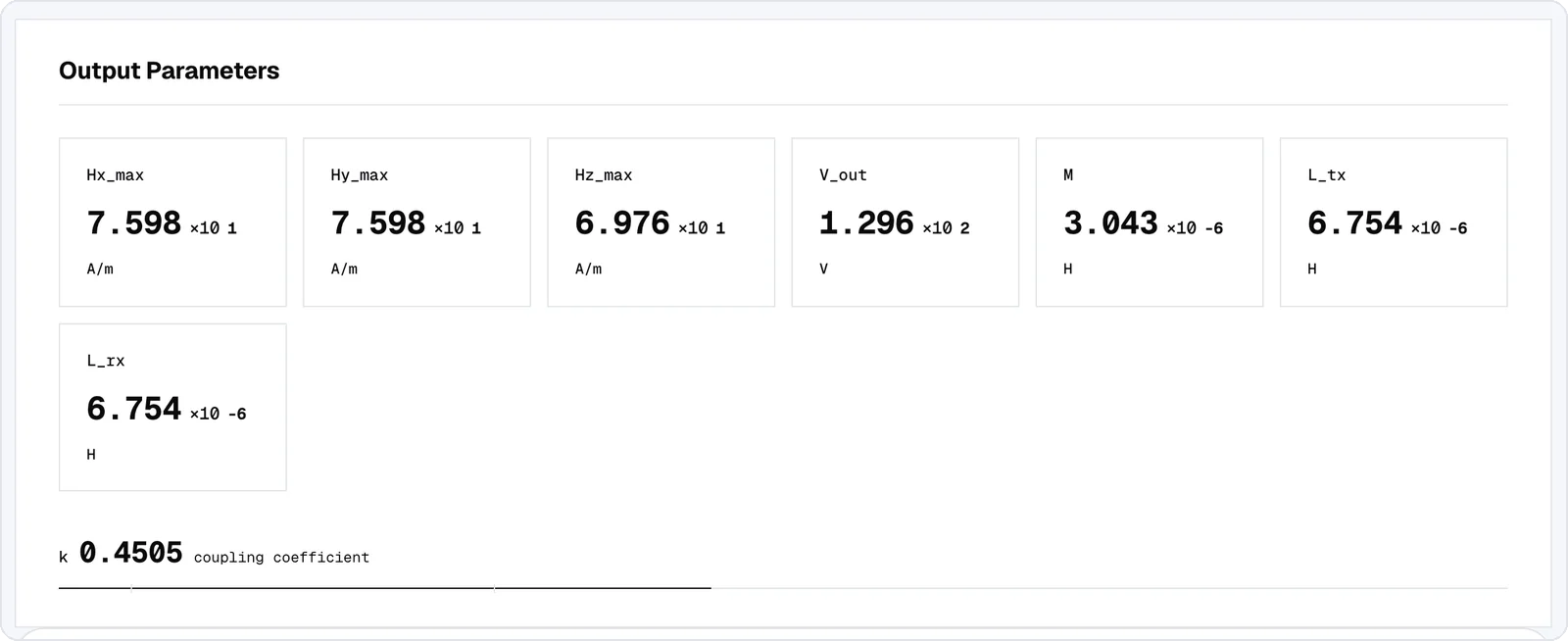
Four square and four circular geometries — Helmholtz–Helmholtz, DTC–Helmholtz, Helmholtz–DTC and DTC–DTC, in both shapes. Each pair has a dedicated calculator with topology-specific input ranges.
- Square: Helm–Helm · DTC–Helm · Helm–DTC · DTC–DTC
- Circular: Helm–Helm · DTC–Helm · Helm–DTC · DTC–DTC
2D, vector, volume.
Switch between a 2D plane heatmap, a downsampled vector-field overlay and a full 3D isosurface volume — all driven by the same H-field tensor. LOD levels 0/1/2 trade detail for a 4× speed-up on heavy grids.
- Modes: 2d_plane · vector · 3d_volume
- LOD: 0 · 1 · 2
Animate the parameter space.
Sweep any of the thirteen tunable inputs — current, frequency, turn count, spacing, coil size — across 2 to 100 steps. Adaptive mode auto-generates ~300 points for smooth efficiency curves. Frames return as a JSON array, ready to scrub.
- Parameters: 13 (I · f · Nr · Nt · h · amax · …)
- Steps: 2 – 100 · adaptive ≈ 300
We show our work.
Coaxial mutual inductance is the Maxwell–Neumann elliptic-integral formula tabulated by Grover (1946) and Babic & Akyel (IEEE Trans. Magnetics, 2008), evaluated directly, so there is no discretisation error to quote. The validation page lists every closed form and what the model does not cover.
- Mutual inductance: closed form (Neumann)
- Field: closed form (Biot–Savart)
- Scope: air-core · magnetostatic
Save once, re-use everywhere.
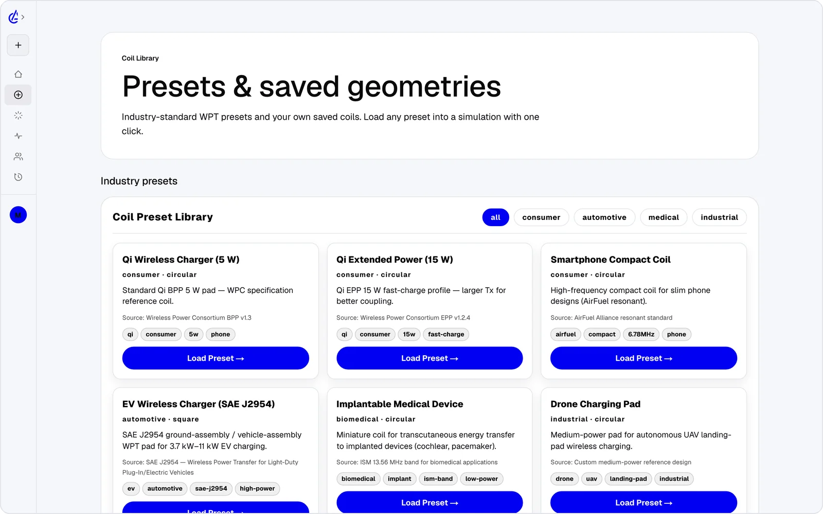
Persist coil geometries to your personal library and pull them into any of the eight calculators. CSV import for migration from a spreadsheet; bulk edit for parameter studies.
- Import / export: CSV · JSON
- Operations: bulk edit
Geometry that finds itself.
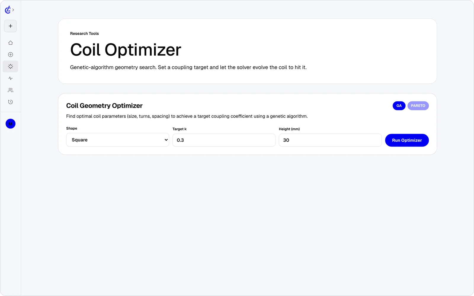
A micro-GA with BLX-α crossover and tournament selection (k = 3) runs 80 generations of population 40 to hit a coupling target. Multi-objective mode returns an NSGA-II-style Pareto front over k, η and power.
- Algorithm: micro-GA · BLX-α
- Budget: 80 gen × pop 40
- Multi-objective: NSGA-II Pareto
From session to fab.
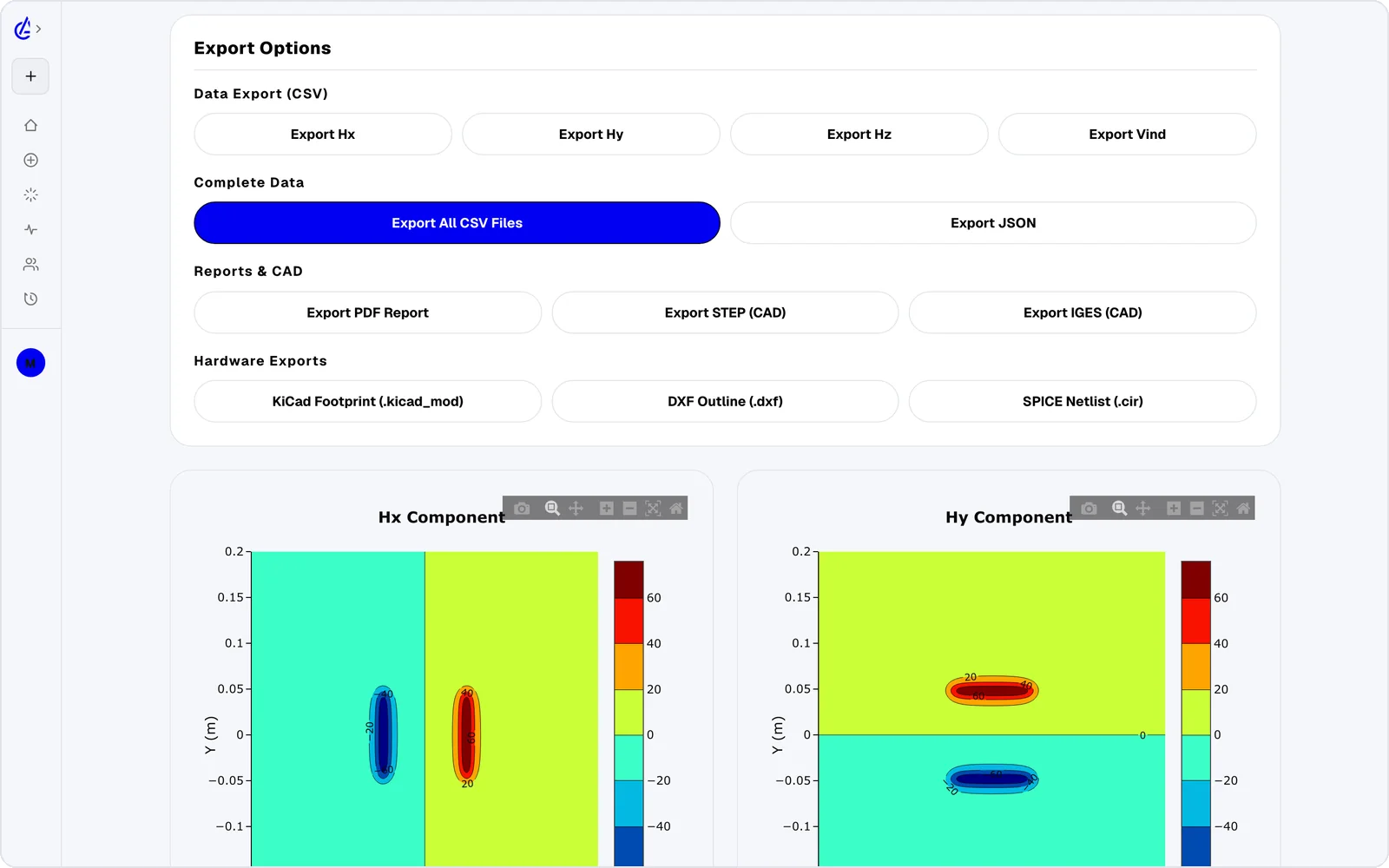
Every run exports four ways: a typeset PDF report, a KiCad PCB footprint (.kicad_mod), a DXF outline for downstream CAD and a SPICE netlist with the L · M · k component values for circuit simulation.
- PDF: report
- KiCad: .kicad_mod
- DXF: outline
- SPICE: L · M · k
One engine, three surfaces.
Run from the web dashboard or the iOS & Android app; a native macOS / Windows / Linux desktop build is coming soon. The 6.78 MHz ISM and 85 kHz SAE J2954 bands ship as presets, and custom frequencies are accepted within the magnetostatic model.
- Platforms: web · iOS · Android · desktop soon
- Bands: 6.78 MHz · 85 kHz · custom