Learn the physics. Ship the design.
A curated path through Biot–Savart fundamentals, the eight-topology workflow and deeper research notes. Built for engineers new to WPT and for practitioners tuning production coils.
Start with first principles.
Biot–Savart from scratch
Derive the magnetic field of a current element and build up to the closed-form mutual inductance of two coaxial loops.
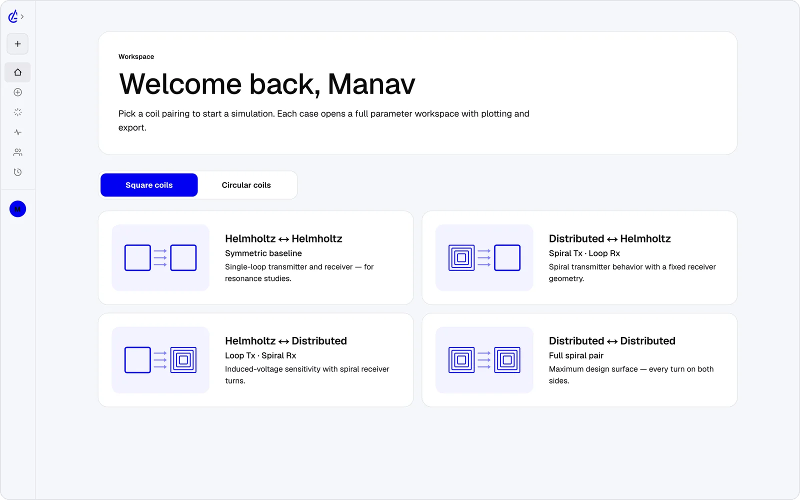
Helmholtz vs DTC
Why the eight topologies look the way they do — uniformity at the centre versus high-coupling at distance.
Coupling factor, k
The single number every WPT design lives or dies on. What it means, how it scales with spacing, and why ½ is hard.
Reference articles.
The Learn hub answers one engineering question per article, with equations, worked numbers and cited sources.
Wireless power coil design guide
Designing a coil pair end to end: topology, size, turns, gap, k, Q, compensation, frequency, exposure limits and fabrication, with worked numbers.
CouplingCoupling coefficient k explained
What k is, how to compute it from geometry, representative values and how it falls with distance and misalignment.
CouplingMutual inductance: Neumann and Maxwell
The definition, the Neumann double integral, Maxwell’s elliptic-integral formula for coaxial loops and a worked example.
FieldHelmholtz coils: spacing and field
Why d = R for circular pairs and 0.5445·side for square pairs, the centre-field formulas and how uniform the field really is.
CircuitWPT compensation topologies: SS, SP, PS, PP, LCC
When to use each resonant network, the design equations, and frequency splitting and bifurcation.
CircuitWPT efficiency and the kQ figure of merit
η_max = U²/(1 + √(1 + U²))², why Q matters as much as k, skin depth and litz wire.
StandardsWireless charging standards and exposure limits
Qi, SAE J2954 and AirFuel Resonant frequencies and power classes, and the ICNIRP and IEEE C95.1 exposure limits.
MethodsBiot–Savart vs FEM for coil simulation
When a closed-form Biot–Savart solver is enough and when you need FEM or full-wave: ferrite, shields, eddy currents, self-resonance, SAR.
Run a real simulation.
Your first simulation in 90 s
Pick a topology. Set geometry. Run. Export. End-to-end on the web app, no setup.
Sweep spacing across 50 frames
Use the parameter-sweep API to render a k-vs-h curve and pin the operating point.
From sim to fab
Walk through the four export targets — PDF, KiCad, DXF, SPICE — and what to drop into your toolchain first.
Inside the solver.
Inside the genetic optimiser
BLX-α crossover, tournament selection, NSGA-II Pareto. How to read the convergence curve and when to restart.
Volumetric field rendering
How the same H-tensor drives 2d_plane, vector_field and 3d_volume modes — and what LOD 0/1/2 actually means.
Validating against Babic & Akyel
How the solver's mutual inductance is checked against the Babic & Akyel closed form for coaxial loops, and where the model stops.
Worked examples by application.
EV pads at 85 kHz
SAE J2954 alignment, gap and misalignment trade-offs. Worked example from a square-DTC ground assembly.
6.78 MHz ISM implants
Sub-mm coil design for medical implants — Q targets, coupling under tissue load, regulatory hooks.
Battery-free IoT sensors
Designing the receive coil when budget is microwatts. Rectifier choice, matching network sizing.